What Is GTO in Poker? A Practical Explanation
An introduction to game theory optimal poker, ranges, mixed actions, and the limits of one declared solver example.
Contents
GTO means game theory optimal. In poker, it is shorthand for a strategy that is designed for a particular game model so that an opponent cannot gain much by exploiting it. It is not a promise that one poker chart, one hand, or one solver screen is best everywhere.
That definition starts with the model. Positions, stack depth, ranges, rake, board, bet sizes, and stopping rule all affect the answer. In imperfect-information games, methods such as counterfactual regret minimization search for an approximate equilibrium of the stated game; they do not make every real no-limit hold'em situation “solved.” Zinkevich et al. (2007) and Bowling et al. (2015) are useful context: the latter's solved claim is for a specified heads-up limit model, not all of no-limit hold'em.
Think in ranges, not one hand
A range is the set of hands a player can plausibly hold, together with their weights. A strategy can mix actions because the range needs protection across actions; that does not mean a player should alternate actions by feel. The practical task is to read the assumptions first, then treat each displayed frequency as an instruction for the named model and node.
For a product view of preflop ranges, see Ranges. For the hosted product's API surface, see the GTO poker solver API guide. The glossary defines terms such as EV, range, and isomorphism without turning this article into API documentation.
A declared root-node example
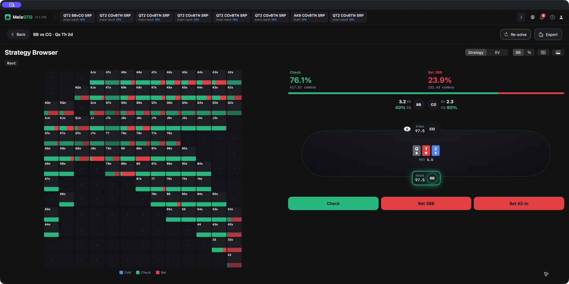
This example uses one real Direct CPU capture with GG200NL 100 bb ranges: 6-max cash, CO opens to 2.5 bb, BB calls, and the flop is Qs Th 2d. The root pot is 5.5 bb and the remaining stack is 97.5 bb. BB is out of position and CO is in position. The applied setup preserves the source ranges' mixed class weights; this is an example input, not a claim about a uniquely correct preflop range or a full GG rake equilibrium.
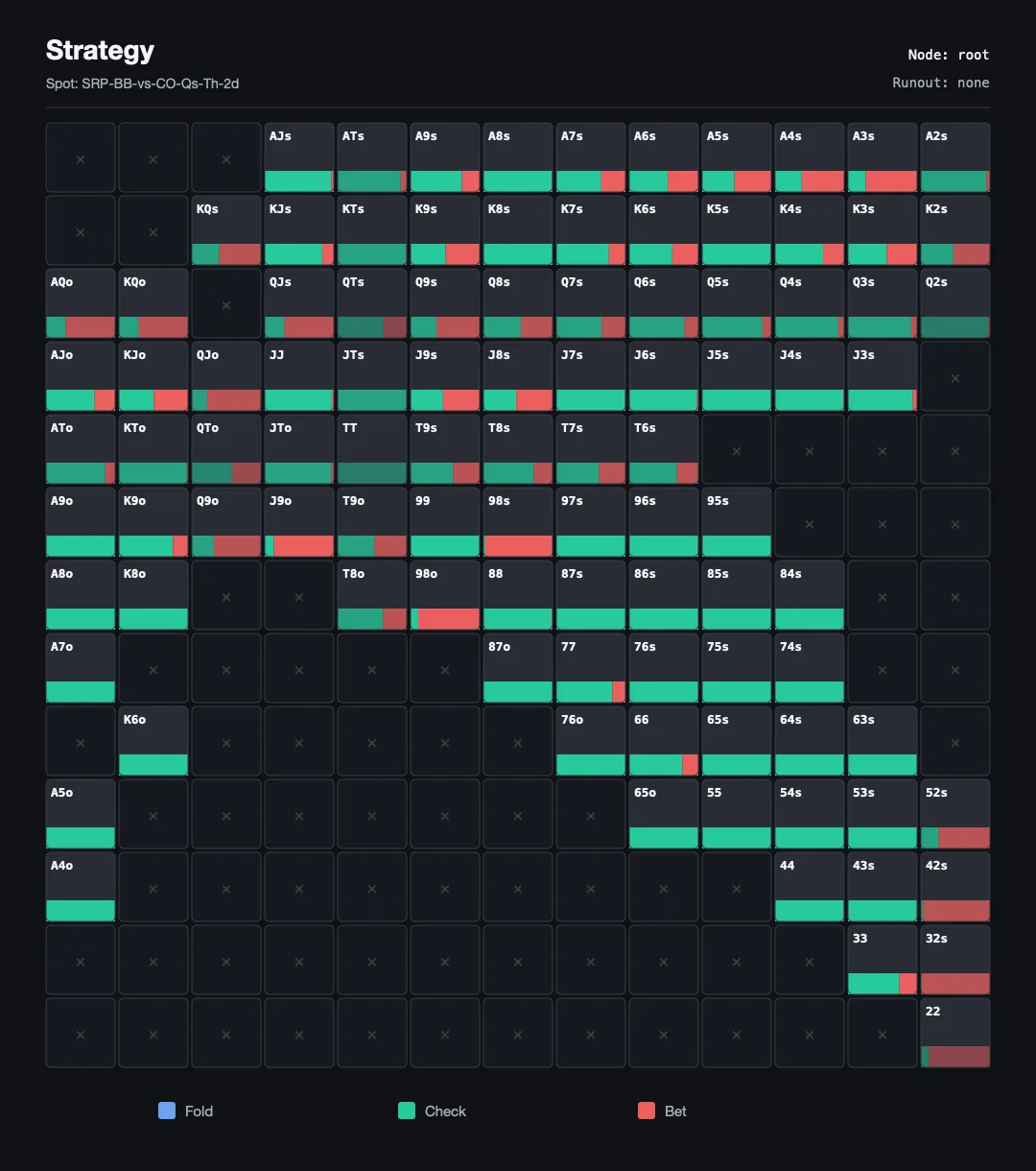
For the KQs class at the BB root, the comparison below uses the native CSV's class-level means. Frequency is the arithmetic mean across surviving KQs combinations; action EV is the corresponding per-action class mean in bb. Neither is a whole-range weighted result, a per-combination EV, equity, or the original preflop KQs weight. The input KQs weight is 0.913, while the CSV's InRange 0.7500 is a surviving-combo coverage fraction.
KQs frequency
KQs class action-frequency comparison from the captured BB root CSV.; Root action; Class frequency
Action EV 3.8028 bb
Action EV 3.7597 bb
Action EV -0.7566 bb
CSV display rounds this action to 0.00%; this is not a strictly zero-probability claim.
| Root action | KQs frequency |
|---|---|
| Check | 0.3978 |
| Bet 3 bb | 0.6022 |
| Bet 97 bb | 0 |
The native strategy export below is an image produced by the app for that BB root node. It is not a desktop screenshot and it is not the source of the values above.
The full English Direct UI screenshot is separate display evidence from the same CSV-bound capture. It is included to show the result surface, not to transcribe metrics from pixels.
What the example does and does not say
The setup configures a 50% pot bet, which is 2.75 bb at this root; native 1 bb rounding makes the actual action BET 3.000000. The root also retains CHECK and BET 97.000000, so this is not a two-action tree. The third action's rounded CSV frequency must not be rewritten as “never bet.”
The capture used CPU, customExact, FP32, maxIteration 100, a configured 0.5% pot accuracy target, and isomorphism. Its postflop tree is a local no-rake-deduction model; it does not claim to reproduce the original GG rake model. It does not expose a final iteration count or measured exploitability. The observed completion time was an upper bound of 98.509 seconds, not an exact solve-time measurement. Those omissions mean this example does not claim that the configured accuracy target was achieved, that the output is a complete equilibrium, or that the line is general advice for another game.
A useful learning workflow
- State the spot before reading a recommendation: positions, stacks, ranges, board, rake treatment, and available actions.
- Identify the node and the statistic. Frequency, action EV, equity, and range-weighted EV answer different questions.
- Preserve small actions instead of deleting them because a rounded display is zero.
- Change one assumption at a time before comparing outputs. A new board or range is a new model, not a continuation of this result.
- Use solver output for study and practice—not real-time assistance in live play.
Inputs and results
This study example is not a strategy prescription. Its inputs were NLHE 6-max, with BB out of position and CO in position: both started at 100 bb; CO opened to 2.5 bb, BB called, and the flop was Qs Th 2d. The root pot was 5.5 bb and the remaining stack was 97.5 bb.
Downloads
- Download the root-node CSV result — 8,495 bytes; 98 BB hand classes with root-node frequencies (0–1 fractions) and action EVs (bb), not a complete tree or per-combination result.
- Download the complete saved input JSON — 3,946 bytes; the exact saved setup used here.
- Download MelaGTO Direct v1.1 (10).
| Setting | Value used |
|---|---|
| Solver | CPU, FP32, customExact |
| Bet sizes | 50% pot for both players on flop, turn, and river; native 1 bb rounding makes the flop half-pot action 3 bb |
| Tree | raiseLimit 1; allinThreshold 0.67; isomorphism enabled |
| Stop configuration | maxIteration 100; 0.5% pot accuracy target; threads automatic (-1) |
The target is a configuration, not proof of attained convergence. The capture does not provide a final iteration count or measured exploitability. Its root still contains CHECK, BET 3.000000, and BET 97.000000; the CSV rounds the third action's frequency to 0.0000, so it is not a claim that the action is impossible.
Ranges used
These are the complete mixed-weight ranges from the saved input, formatted for Direct's Bulk edit fields. Classes and weights are preserved to three decimals; unlisted classes have weight 0.
BB OOP (98 classes)
22:1.000, 33:1.000, 44:1.000, 55:1.000, 66:0.900, 77:0.965, 88:0.956, 99:0.920, 32s:0.431, 42s:1.000, 43s:0.804, 52s:1.000, 53s:0.873, 54s:0.727, 63s:1.000, 64s:0.711, 65o:0.060, 65s:0.706, 74s:1.000, 75s:0.871, 76o:0.176, 76s:0.665, 84s:0.309, 85s:0.949, 86s:0.916, 87o:0.163, 87s:0.746, 95s:0.387, 96s:0.927, 97s:0.928, 98o:0.271, 98s:0.823, A2s:0.711, A3s:0.735, A4o:0.289, A4s:0.754, A5o:0.815, A5s:0.540, A6s:1.000, A7o:0.849, A7s:1.000, A8o:0.928, A8s:1.000, A9o:0.996, A9s:0.998, AJo:0.937, AJs:0.785, AQo:0.912, ATo:0.951, ATs:0.883, J3s:0.828, J4s:0.885, J5s:0.936, J6s:0.875, J7s:0.731, J8s:0.747, J9o:0.482, J9s:0.334, JJ:0.224, JTo:1.000, JTs:0.384, K2s:0.912, K3s:0.652, K4s:0.747, K5s:0.882, K6o:0.083, K6s:0.921, K7s:0.856, K8o:0.101, K8s:0.995, K9o:0.980, K9s:0.814, KJo:0.779, KJs:0.527, KQo:0.700, KQs:0.913, KTo:0.856, KTs:0.772, Q2s:0.815, Q3s:0.818, Q4s:0.805, Q5s:0.701, Q6s:0.622, Q7s:0.997, Q8s:0.611, Q9o:0.452, Q9s:0.499, QJo:0.906, QJs:0.145, QTo:0.926, QTs:0.577, T6s:0.829, T7s:0.915, T8o:0.057, T8s:0.910, T9o:0.839, T9s:0.265, TT:0.808
CO IP (73 classes)
22:0.417, 33:0.407, 44:1.000, 55:1.000, 66:1.000, 77:1.000, 88:1.000, 99:1.000, 54s:0.302, 65s:0.401, 76s:0.357, 87s:0.566, 97s:0.623, 98s:1.000, A2s:1.000, A3s:1.000, A4s:1.000, A5o:0.926, A5s:1.000, A6s:1.000, A7o:0.464, A7s:1.000, A8o:1.000, A8s:1.000, A9o:1.000, A9s:1.000, AA:1.000, AJo:1.000, AJs:1.000, AKo:1.000, AKs:1.000, AQo:1.000, AQs:1.000, ATo:1.000, ATs:1.000, J7s:1.000, J8s:1.000, J9o:0.305, J9s:1.000, JJ:1.000, JTo:1.000, JTs:1.000, K3s:1.000, K4s:1.000, K5s:1.000, K6s:1.000, K7s:1.000, K8s:1.000, K9o:0.677, K9s:1.000, KJo:1.000, KJs:1.000, KK:1.000, KQo:1.000, KQs:1.000, KTo:1.000, KTs:1.000, Q5s:1.000, Q6s:1.000, Q7s:1.000, Q8s:1.000, Q9o:0.213, Q9s:1.000, QJo:1.000, QJs:1.000, QQ:1.000, QTo:1.000, QTs:1.000, T7s:0.670, T8s:1.000, T9o:0.160, T9s:1.000, TT:1.000
Use the JSON as the complete parameter reference: in Direct, create a Custom spot with the values above, paste the full ranges with Bulk edit, choose CPU solving, and compare the root-node output with the downloaded CSV. Version, hardware, and stopping conditions can affect an exact rerun.